(Update: New architecture with better results here)

So after a few weeks of chugging away at lots of different model/parameter combinations I’ve settled on an architecture that performs reasonably well on the task I described in the last post. Namely, given a sequence of glimpses $w_t$ of a 3D model, generate an image $I$ of that model from a given viewpoint $p$.

First I’ll get into the architecture I used to accomplish this and then describe the various tricks that had to go into this to get the results halfway decent.

Architecture

In all the experiments I used 4 glimpses of each (3D) model as inputs to the network. An important difference from my last experiment is that the glimpses are prerendered instead of during training time which greatly speeds up training time. Each 64x64 image is first encoded with a 3 layer convolutional network with {32,64,128} feature maps in each layer, with ReLU activations and max pooling. The result is a 128x8x8 map $x_enc$ for each image. This map is flattened and passed through a linear transformation and a ReLU layer to obtain the feature vector $g_x$.

The 4D viewpoint coordinates (r,theta,z,z_look where the first 3 are the normalized cylindrical coordinates of the camera pointed at the z axis and and the 4th is the point on the z axis where the camera is pointed) $l$ are transformed into a vector $g_l$ after a linear transformation and a ReLU layer.

And the two vectors $g_x$ and $g_l$ are concatenated into feature vector $g$.

These vectors are passed into an LSTM

The tricky part is then to take this final vector $h_T$, which we want to contain information about the 3D shape of the object, with the desired viewpoint $l_{out}$ and generate an image. A few resources (¹) have suggested multiplicative interactions for combining separate pieces of information so I went with a slight variation on that. First the output viewpoint $l_{out}$ is transformed into a higher dimensional vector through a linear transformation and ReLU activation

This new vector is then transformed into two new location vectors vectors $g_{l1}$ and $g_{l2}$

With the linear maps being independent of one another. The shape vector $h_T$ is passed through a ReLU layer with output size the same as the location vectors.

The network then combines the shape and location information as follows:

This is inspired by the form of the perceptron with one hidden layer. Intead of linear transform -> nonlinearity -> linear here we have element-wise product -> nonlinearity -> element-wise product, with the product parameterized by the 4D location coordinates. This should allow the transformation applied to the shape vector to be more complicated. Finally the $h_out$ vector is transformed one more time and reshaped into a 12888 map. This is then passed into a 3 layer decoder which has a symmetrical architecture to the encoder. This encoder produces the final image. This is compared to target image taken at viewpoint $l_{out}$ with a squared error criterion

The error from this criterion is then propagated back through the entire network. The Adam algorithm was used for optimization.

Tips and Tricks for Training

Data Augmentation

I’ve been working with the Princeton Shape Benchmark dataset which has a fairly wide variety of models but only contains about 1000 of them which as far as “Big Data” is concerned is not very big at all. This can be remedied somewhat as 3D models lend themselves very well to augmentation. Before each set of renders is taken (4 initial glimpses and then the target renders) the model is rotated and scaled by a random factor, and multiple render sets of each model are taken to artificially enhance the size of the training set.

Space Filling

Instead of using a PRNG to sample viewpoints from which to generate target images I generated quasirandom numbers to ensure the coordinate space was covered as fully as possible. NAME has a great post on quasirandom sequences if you want to read more about them. I used a Halton sequence to generate values of theta and z, keeping r and z_look constant to simplify the problem somewhat.

Dropout

This is one of the best known regularization techniques right now so I don’t have too much to say about it. Dropout after the second convolutional encoder layer helped reduce overfitting but adding dropout to additional layers further slows convergence without seeming to help validation/test performance much or at all.

Batch Normalization

Batch Normalization helps alot with convergence but should be used carefully. For a week or so the network wouldn’t learn anything but an average of the target images until I removed Batch Normalization from the combining portion of the network (g_l1 and g_l2 layers). I’m still not entirely sure why this was the case but it seems like constraining vectors that are being multiplied together to be normalized restricts the range of functions it can represent.

Auxiliary Training

Since the output shape of the encoder map is the same as the input shape of the decoder, I can give those two parts of the model a separate task to help these two components learn good features. The output of the encoded glimpses is fed into the decoder, which tries to recreate the original image. So this is basically training an autoencoder in addition to the full network. The gradients from this are multiplied by a small multiplicative factor and added to the full gradient before the parameters are adjusted.

Results

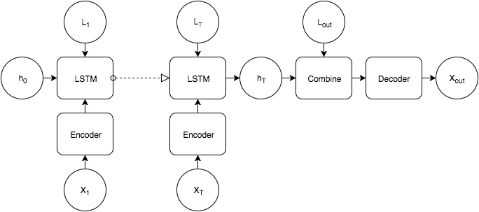
Samples from the training set compared against their training targets:

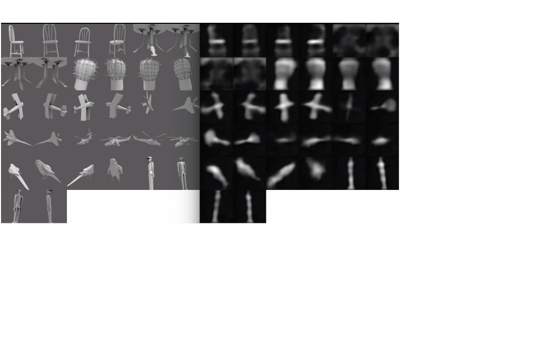
Samples from the test set and the targets they’re trying to match:

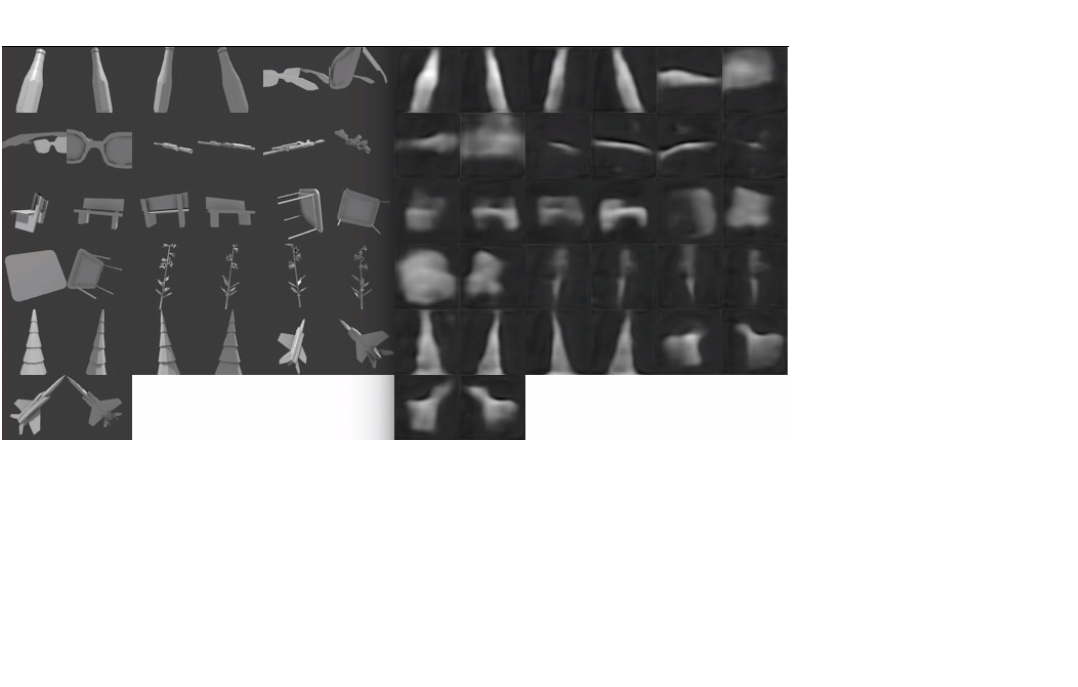
Early stopping was used so training was stopped as the squared error reached about .0029 per pixel on the validation set even as the training error continued to improve. The space of all 3D models is much too wide to be captured with only 1000 or so examples no matter how much you augment the data. The model would most likely perform much better if trained on some small subset of objects, like just houses, and was used to only encode houses. The distributions of the test and training sets are bound to be fairly different due to the small sample size but the model does an ok job of learning a general shape for simple objects. It’s difficult to capture the finer features of the object with a flat vector of only 1024 dimensions but for the less complicated shapes the network does a good job of learning a general function for foreshortening based on viewpoint and knowing which side of the object to show if the two sides are wildly different.

So the model does a good job of generalizing over viewpoints and an ok job of generalizing over objects. This is expected as augmentation can provide infinite viewpoints but only a very small fraction of possible objects.

Future Improvements

More data is going to improve the results and reduce overfitting 99 times out of 100, so if anyone knows of a similar freely available dataset which contains lots of 3D objects of various types let me know.

I also think that by flattening the feature maps and then going back to a 3D tensor makes it hard to recover the spatial information. I hadn’t thought of a good way to combine an LSTM type model with convolutional nets but looking at the recent success of Neural GPUs ² it seems like a similar architecture could really improve my results. Look out for my next blog post and I’ll tell you if it works. I promise I’ll tell you even if it doesn’t.