Learning 3D Shape (1)
In the past few years we’ve come a long way towards training algorithms to classify natural images. While being able to tell which breed of dog is the object of interest in an image is certainly not ‘understanding’ the way you or I understand the visual world, it’s no small feat to be able to compete with or outperform human classification accuracy on a dataset like ImageNet. This can’t be achieved by looking at only surface level features and in some sense the model has to learn ‘deep’ features about an object that generalize to many different positions/sizes/lighting conditions.
Another task humans seem to be good at is inference of 3D shape. Yes we have binocular vision but even with one eye closed if you look at an object from one angle typically you can take a reasonable guess as to what the object will look like from another angle, incorporating prior knowledge about the object itself and about 3D shapes in general. The hypothesis for the next few blog posts is that we can train a model to do this kind of inference the model will have a general ‘understanding’ of how 3D shapes behave under perspective transformations which may prove useful for classification/generation tasks.
More formally, we want a function
where is a variable referring to the position of the observer and is the set of previous position/image pairs. So, given a set of images and the positions those images are from, predict what the image will be at a new position .
Shape Classifier
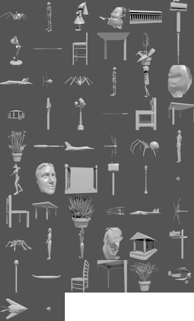
Before tackling this problem I tried to solve a somewhat simpler and more recongnizable problem. Given the set of image position pairs, predict the class of the object. For a dataset I used the Princeton Shape Benchmark dataset of 3D models1. Using 3D models allows us to augment the data easily through rotation, scaling, and translation operations.
An algorithm I’ve been wanting to implement for a while is the Recurrent Attention Model (RAM) from a paper by Mnih et al.2 This algorithm, instead of processing a whole image at once, will take a glimpse of a portion of the image and pass that into a Recurrent Neural Network. At each step the RNN will output the next location for the “glimpse sensor” to move to. At the last step the network will predict the image class based on the recurrent state. It was fairly straightforward to adapt the algorithm to work with 3D objects. The location of the glimpse sensor becomes the position of the camera and the glimpse becomes the full image rendered from the given camera location.
The network can predict any potential camera location within a given range, but we can’t render an image for every possible camera position in advance. So what I really should have done was take maybe 100 or 500 or a million renders for each object from different camera positions and feed the network the render whose position matches the network’s position output the closest. Here’s what I did instead…
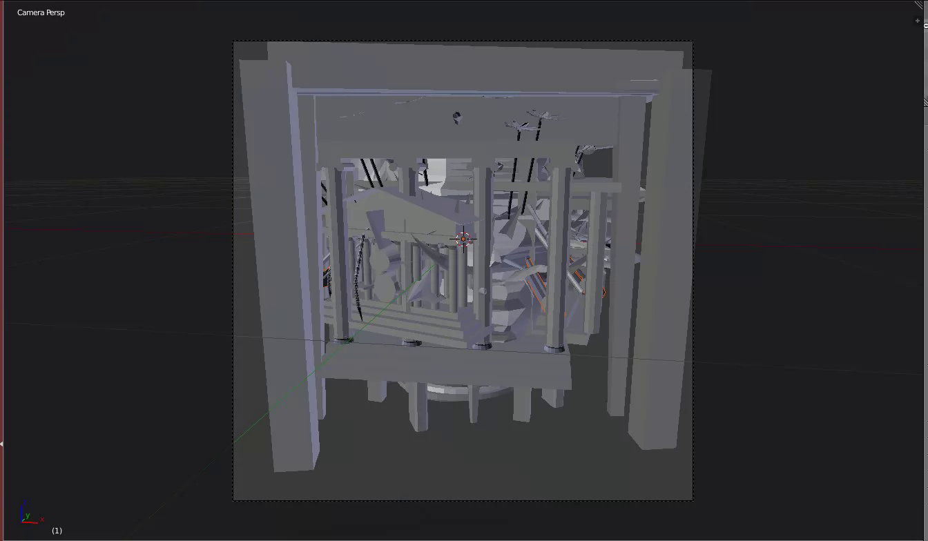
I loaded all the .off models from the Princeton dataset into Blender (a 3D modeling tool) and saved them down in batches. Then I set up a simple python http server inside Blender which could receive commands to position the camera at a certain position and render one of the models. (Ok the http server isn’t really that simple to get it to work inside python but all of the hard work was done by akloster3. I just built a little bit on top of it.) These renders are then all taken in to the network as a batch and then the network outputs the locations of the next renders which are then sent over to the Blender server and the process repeats. So for each object for each camera position the Blender process will render a new image on the fly and save it down. This is terribly inefficient for a number of reasons, but at least it looks cool.
One advantage of doing things this way though is that it’s super easy to augment the data. Every time a batch of models is loaded into Blender each one is rotated by a random amount around the Z axis and has a small scaling performed along each of its axes. The network never sees the same example twice.
Model and Details
So the actual model I used, if you don’t want to dig through the mess of code in github, is as follows:
Input image x is 1x64x64 (grayscale)
is obtained from x by passing x through a series of 5x5 convolution layers followed by Rectified Linear Units (ReLU) followed by 2x2 max pooling. Here is used 3 layers with 64,96, and 128 feature maps in layers 1,2,and 3, respectively. The final layer is 128x4x4 and is flattened into a vector .
Where Linear means a linear transformation plus a bias vector, is the 4D vector containing camera position output by the previous step. The first 3 component correspond to the position of the camera in cylindrical coordinates (within a multiplicative factor to keep the values between -1 and 1). The camera is fixed to always point at the z axis and the 4th component of the location vector refers to the height of the point on the z axis the camera looks at.
(Other papers suggest multiplicative interactions instead of concatenation and passing through a Linear/ReLU layer. Something to try.)
Then the vector g is passed into an RNN
At each step the network predicts the location for the next render
where between -1 and 1 and takes a value of 1 when x > 1 and -1 when x < -1. After T steps the network will predict the class of the object.
Results
So for a while this didn’t really work at all. I was getting maybe 50% accuracy on the training set and comparable results on the validation set. This may sound ok but I used the set of classifications on the Princeton Shape Benchmark dataset with the lowest granularity. There were only 7 classes. Vehicle, animal, household, building, furniture, plant, other. I actually think this may make it harder for the classifier to predict rather than easier. How the classifier is expected to understand that a face is Other but a whole person is Animal is beyond me. At the same time the dataset is relatively small, with only about 1000 models in the test set, so a more fine grained categorization would leave a pretty small number of examples for each class.
But what made me think this was more an issue with the model architecture than lack of data or poorly classified images is that I wasn’t able to overfit to the training set. With the number of glimpses set to 1 the model can overfit just fine but with 2 or more glimpses the RNN isn’t able to properly send the gradients back to the convolutional layers for them to learn meaningful features. I tried a bunch of variations on number of RNN layers, LSTM versus standard Elman net, number of hidden units in each layer, number of fully connected layers after the convolutional layer, nothing seemed to really get the training set accuracy above 50 or 60%. And if you cant fit to your training set there’s really no hope for the test set.
I had remembered the idea of “auxiliary training” mentioned in this paper by Peng et al.4 They faced a similar issue with weak supervision and a relatively small dataset size, so in addition to the error from the task the network is trying to accomplish, they train another network to reconstruct the original input from the task-specific representation. The idea is that this encorages good feature selection, similar to how initializing the weights of a classifier by first training an unsupervised model can sometimes lead to better results.
I implemented this by reconstructing a downscaled version of the original image from the vector
The vector is first passed through a linear layer and then reshaped into a 128x4x4 collection of feature maps. Then I apply upscaling transformations and convolution layers until the image is the appropriate size before a final 1x1 convolution to get the final pixel output.
Surprisingly, this seems to work. Using two glimpses for each object, the network is able to train the test set to 92% accuracy after about 200 epochs. If I had let it run longer it probably could have fit almost 100% of the inputs. This is actually a pretty decent result due to the significant augmentation done on the data. The model’s not just memorizing the 900 or so objects but has to actually learn features that generalize at least across different transformations of the same object. The validation set gets about 63% accuracy. I haven’t run the network on the test set but I’m assuming it will be about the same. Due to the small amount of data I don’t know if it could really do much better. If the training set contains a bunch of insects and no horses there’s a horse in the test we can’t reasonably expect the model would be able to learn it. The space of all 3D models is simply too large to be learned with only 900 examples.
Still there is room for improvement. For one thing, when you look at the “reconstructions” generated by the auxiliary net they don’t really look like anything at all after 200 epochs.
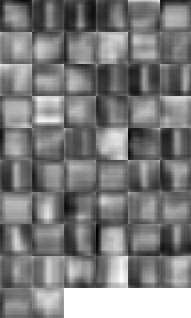
So it’s not really clear to me why this helps with the training. I suppose passing a signal through the network at each step as opposed to one supservised signal passing through the entire chain of steps is easier to learn from. I have a feeling it’s learning to reconsturct as best it can with the architecture I’ve set up for the reconstruction net. Upscaling by doubling feature map width/height and replacing each unit with the same values copied into a 4x4 square seems like a bad way to go about it. Next steps are to look into some Convolutional Autoencoder(CAE) implementatons and try and train one. Maybe pretrain the reconstruction net as the decoder to a CAE, which could speed up the learning and lead to a lower test error.
Anyway I’m fairly happy with the classifier which was really only an exercise to develop the architecture needed to work on the shape inference problem so the next post will be about that.